QuickCSG is also available as command-line executables (v2.1) that don't require compilation:
Linux x64 (compiled on Debian 7): mesh_csg_linux.
The parallel version mesh_csg_linux_tbb requires the TBB dynamic library to
be accessible, use your favorite package manager to install it.
mac (OS X 10.9 64 bit): mesh_csg_mac. If you have
installed TBB, eg. via macports, the parallel version is here mesh_csg_mac_tbb.
Windows (Win 7, 64 bit): mesh_csg_win.exe. No multithreaded version yet, and the code is compiled by VC++, which may be a bit slower than gcc on Linux.
The main command-line arguments are: the filenames of the input
meshes, the name of the output (with -o) and the CSG
operation to execute (like -union, -inter or -min2).
Many other options exist, call with -h to list.
Mesh I/O is done in the
simplistic OFF
file format by default. It can be read/manipulated/converted by
eg. Meshlab.
By default mesh_csg is not verbose. Logging is controlled
via the -v option. Most often -v 1111111
gives a pretty good idea of what is going on. Verbosity can be
increased for some stage by replacing one of the '1's with a higher number.
Setting verbosity to the maximum can easily generate hundreds of megabytes of text.
This executable is limited to 63 input meshes (this is a compile-time option).
By default the generalized polygons output by the algorithm are not tesselized:
all vertex loops are returned as polygons in the OFF file,
even when they correspond to holes. Most viewers will not display the OFF correctly
(in fact it is an invalid OFF file).
The -tess3 uses the GLU tesselizer to produce only triangles on ouput,
and -tess produces convex polygons.
The facets of the ouput OFF file are colored according to the input
mesh they came from. A useful option is -combined xxx.off
that stores the input meshes in a single ouput file with the correct
face colors and vertex/face indices that correspond to the ones listed in
the logs.
Do not hesitate to give us feedback on the usage performance, bugs, etc. of QuickCSG.
The exectuable is provided only for research and testing purposes. If
you want to see the source, use it in products, etc. contact us.
There is also a version of QuickCSG that supports self-intersecting
meshes. Contact us if you are interested.
Degenerate cases and error handling
QuickCSG relies on the hypotheses on the input
meshes (non-degeneracy and watertightness), and on their configuration (non-coincidence of the
faces of different meshes). Simple meshes
modeled by humans tend to have degenerate configurations (tangent faces, aligned edges, etc.).
Also, many large meshes just happen to have local errors: missing triangles, small self-intersections, etc.
The approach in
QuickCSG is to record the errors that are encountered during processing
and report them, while still producing a possibly incomplete output mesh.
Most errors belong to the following classes:
invalid inputs (self-intersecting or non-watertight meshes) can have
catastrophic consequences if a self-intersecting facet is used
to determine the mesh position of a KD-tree node and causes a useful
node to disappear. ``Catastrophic'' means that the extent of the error can be arbitrarily large.
degeneracies cause some output vertices not to be found, which in
turn produces ``incomplete loops'', ie. the algorithm cannot produce the
corresponding facet. Therefore, the output mesh is not watertight. The workaround
is to randomly translate the meshes independently: -random.translation 1e-4
translates each mesh by a random vector drawn uniformly from [0,1e-4].
The random translation is reverted, ie. the true intersection vertices are recomputed from the faces they
are the intersection of.
since the KD-tree is axis-aligned, axis-aligned facets may also
produce degeneracies. A simple workaround is to apply a random
rotation (-random.rotation) to the input and revert
this rotation at the end.
The examples below sometimes include these random transformations.
Known bugs
The executable cannot parse OFF files that use the comma ',' as a decimal
separator and fails with an unclear assertion about "ret == 3".
Meshlab is able to display those. To fix the input OFF file, replace ',' with '.' using eg.
tr , . < input.off > output.off
The executable cannot do CSG operations of a mesh with itself (eg. B inter B with B a box).
This is a heavily degenerate configuration that does not produce a satisfying result even
with the workarounds suggested in Section 1.1. For this type of operations on small degenerate meshes
CGAL is definitely a better choice.
QuickCSG is picky on the type of meshes it can handle as
input. Each input file should be not be self-intersecting, should be
a manifold, should not contain 0-surface facets. Also, a vertex
should not be at the top of two separate pyramids, which means that
the output of a XOR produced by QuickCSG itself should not be input again to QuickCSG...
Most of these restrictions can be circumvented in pre-processing steps to QuickCSG.
Examples from the paper
We provide input meshes and mesh_csg command lines for
most of the experiments in the paper, as well as some comments and
images that did not fit in the paper. For most images, a larger
version can be seen by opening it in a page of its own. Most images are
snapshots of Meshlab. For some meshes we also provide a link for
visualization with X3D-enabled browsers.
Note that the hierachy and OpenSCAD
experiments rely on QuickCSG's Python
wrapper. We do not provide this interface, so the corresponding
experiments are not reproduced here.
Most complex meshes originally come from
the The
Stanford 3D Scanning Repository. When a lower resolution of a mesh
was required for comparison with other experiments, we used Meshlab's "Quadric Edge
Decimation" tool to reduce the facet count.
T1, T2, H
These are the main test cases of the paper. They were chosen to have
many meshes that intersect very often, to stress the algorithm.
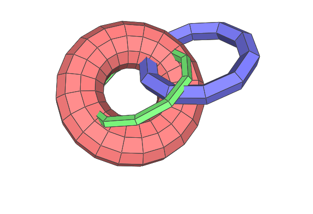
T1: a set of 50 random toruses. We compute difference between the
union of the 25 first toruses with the union of the 25 next ones.
This is a typical CSG case, where there are
many intersecting facets, but the geometry is regular (small
compact facets).
Input and output for T1. Many intersecting facets are tesselated to triangles because they are non-convex:
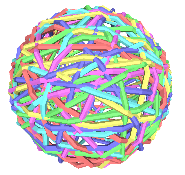
T2: a set of 50 concentric narrow random toruses. The toruses follow
the great circles on a sphere, so each torus intersects each other
torus in two locations. We compute the volumes where at least 2 of
the toruses are present. In this case, most
facets intersect another. This generates many disconnected components
with many more facets than there are on input.
Input and output for T2 (see also the X3D version):
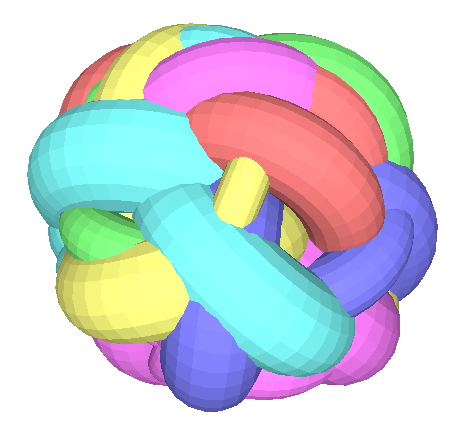
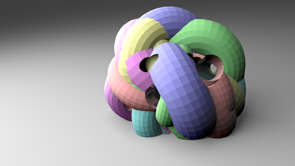
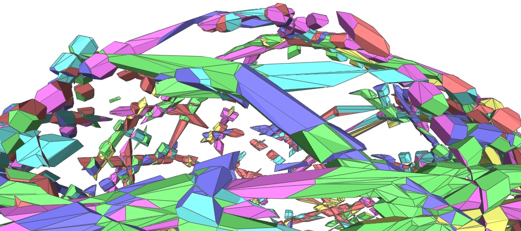
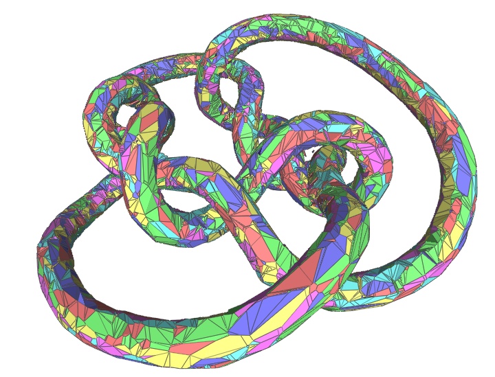
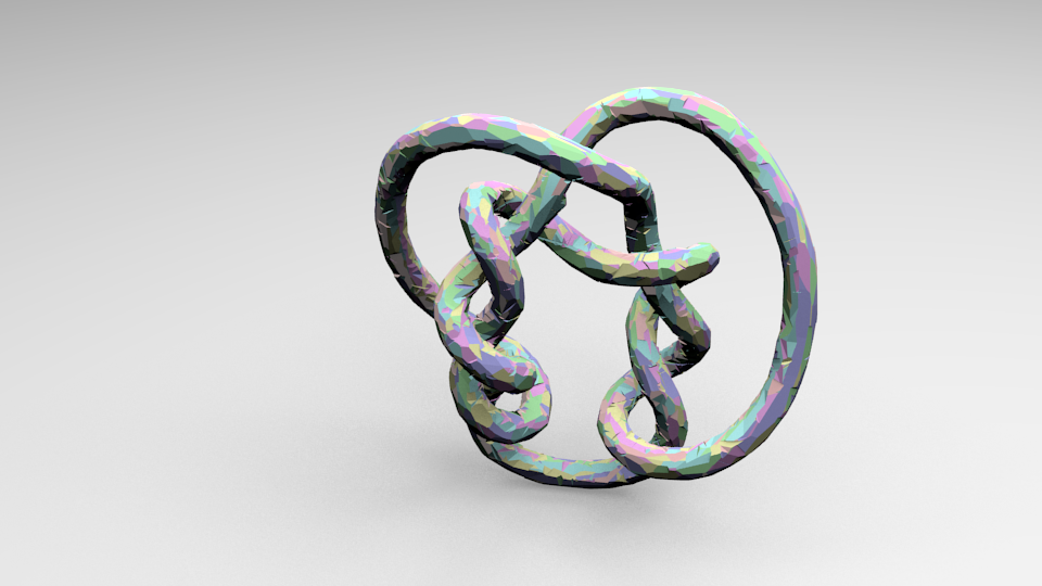
H: a set of 42 visual hulls (projected silhouettes of the object) of
a piece of rope seen from 42 cameras. The facets are very elongated, and there are no primary
vertices in the output mesh. By intersecting these silhouettes the object (a knot) is
reconstructed. The data comes from the original EPVH paper
and the original model from Surface reconstruction from unorganized points paper. Input and output for H:
The meshworks exectuable from the webpage runs on
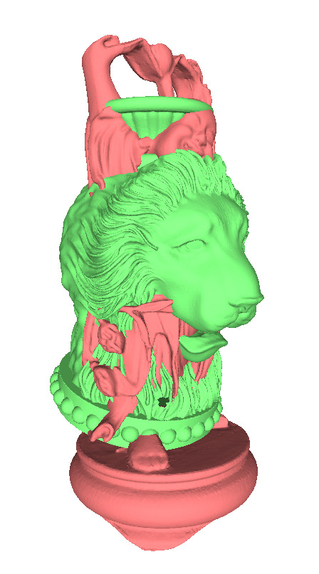
Windows. Here we reproduce some big experiments from the paper, see its Figure 17.
The lion-vase mesh was sent via personal communication, thanks Charlie!
Note that both meshes produce errors. They are due to non-watertight input meshes.
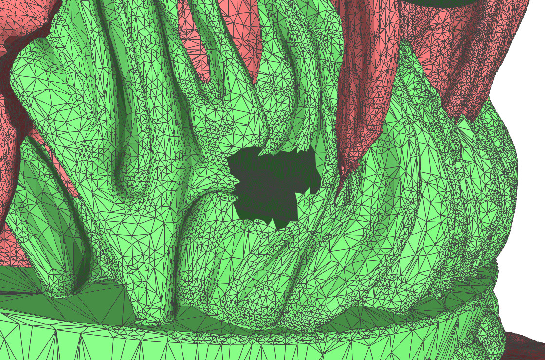
Buddha U lion example. Notice that there is a hole in the mesh.
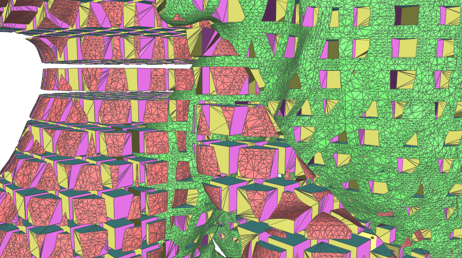
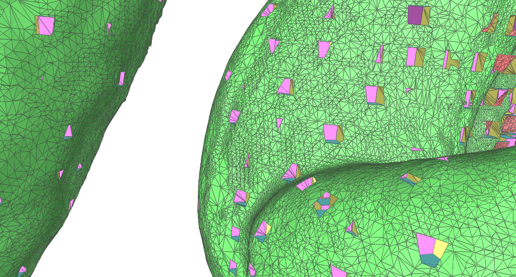
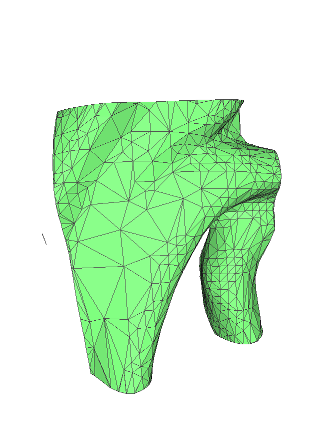
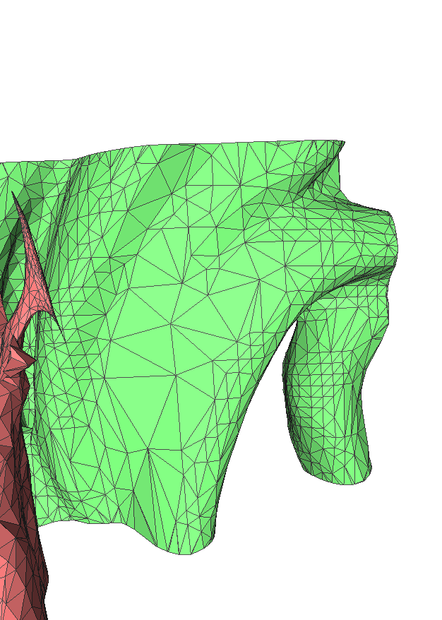
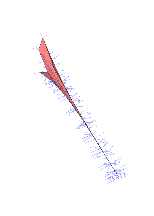
Debugging the CSG error.
a: The hole comes from a KD-tree node. Notice the tiny triangle(s) on
the left of the green mesh. b: this is the parent node. The triangle
comes from an extremity of the red mesh. (c) zoom on the extremity
showing the normals. There is a degeneracy on this small detail, that
was used to decide if the KD-tree node should be cancelled.
(a)
(b)
(c)
./mesh_csg data/cmp_meshworks/{buddha.off,lion.off} -union -o /tmp/out.off -tess -v 1111111
Loading data/cmp_meshworks/buddha.off (off)
Loading data/cmp_meshworks/lion.off (off)
Load input 1907.161 ms
2 meshes, 743526 vertices, 1487474 facets
Register edge-facet links
topology time 335.312 ms
KDTree to vertices
exploration in 542.966 ms
Building output facets
facet time 170.886 ms
Encountered errors during CSG computation:
179 times makeFacetOnlyPrimaries: not same nb of primary vertices as in input
209 times makeFacet: could not find closed loop
93 times addHEPairsPrimary: duplicate facet in primary vertex
2 times addHEPairsPrimary: primary vertex from < 3 facets on output mesh
Storing output /tmp/out.off
output time 1647.991 ms
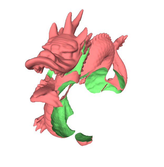
./mesh_csg data/cmp_meshworks/{dragon_277k,bun_zipper}.off -diff 1 -o /tmp/out.off -tess -v 1111111
Loading data/cmp_meshworks/dragon_277k.off (off)
Loading data/cmp_meshworks/bun_zipper.off (off)
Load input 724.481 ms
2 meshes, 174341 vertices, 346632 facets
Register edge-facet links
topology time 81.362 ms
KDTree to vertices
exploration in 120.475 ms
Building output facets
facet time 44.913 ms
Encountered errors during CSG computation:
272 times makeFacetOnlyPrimaries: not same nb of primary vertices as in input
417 times makeFacet: could not find closed loop
102 times addHEPairsPrimary: duplicate facet in primary vertex
18 times addHEPairsPrimary: primary vertex from < 3 facets on output mesh
Storing output /tmp/out.off
output time 370.751 ms
Debugging the missing patch in the mesh:
./mesh_csg data/cmp_meshworks/{buddha.off,lion.off} -union -o /tmp/out.off -tess  -v 1111111 -combined /tmp/combined.off

# out.off misses a part, open it side-by-side with combined, use the
# info tool of Meshlab to see what is missing: vertex 606647

./mesh_csg data/cmp_meshworks/{buddha.off,lion.off} -union -o /tmp/out.off -tess  -v 1111111 -combined /tmp/combined.off -followvertex 606647

# this indicates that the vertex was last seen in node <1221112111211>.
# save the node to an off file:

./mesh_csg data/cmp_meshworks/{buddha.off,lion.off} -union -o /tmp/out.off -tess  -v 1111111 -combined /tmp/combined.off -savenode "<1221112111211>" /tmp/node.off

# what? is this mini-snippet deciding what to do with the green patch?
# How could that happen? Let's see the parent, then the grand-parent.

./mesh_csg data/cmp_meshworks/{buddha.off,lion.off} -union -o /tmp/out.off -tess  -v 1111111 -combined /tmp/combined.off -savenode "<12211121112>" /tmp/node_parent.off
Examples from [Feito 2013]
We reproduced the experiments from the paper as best as we could.
The dragon input mesh is the standard version from the Stanford repository.
The armadillo is a version reduced to 150k triangles. Each one is transformed
so that, between the original and transformed versions,
"The overlapping between meshes has been maximized, in order to achieve a high number of triangle intersections. "
We attempted to reproduce this behaviour in our tests.
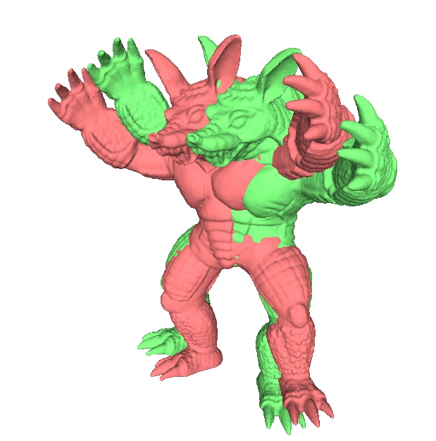
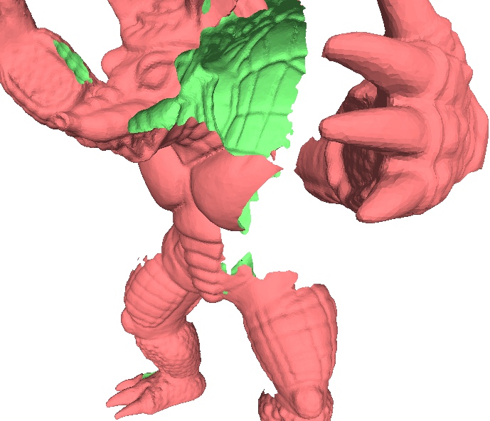
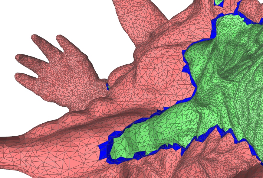
Union, diff, and closeup on diff where non-primary faces are painted in blue:
We did not attempt to exactly reproduce the transformation used in the original paper.
Note that in this example, like for many meshes that have fewer intersections than input facets, i/o time
for the OFF files is dominant.
./mesh_csg data/feito2013/Armadillo_150k.off data/feito2013/armadillo_transformed.off -inter -o /tmp/armadillo_inter.off  -tess -v 1111111111
Loading data/feito2013/Armadillo_150k.off (off)
Loading data/feito2013/armadillo_transformed.off (off)
  Load input 389.010 ms
  2 meshes, 150004 vertices, 300000 facets
Register edge-facet links
  topology time 91.612 ms
KDTree to vertices
  exploration in 133.335 ms
Building output facets
  facet time 39.943 ms
Storing output /tmp/armadillo_inter.off
  output time 222.666 ms

./mesh_csg data/feito2013/Armadillo_150k.off data/feito2013/armadillo_transformed.off -union -o /tmp/armadillo_union.off -tess -v 1111111111
Loading data/feito2013/Armadillo_150k.off (off)
Loading data/feito2013/armadillo_transformed.off (off)
  Load input 390.234 ms
  2 meshes, 150004 vertices, 300000 facets
Register edge-facet links
  topology time 91.419 ms
KDTree to vertices
  exploration in 145.096 ms
Building output facets
  facet time 59.844 ms
Storing output /tmp/armadillo_union.off
  output time 468.811 ms

./mesh_csg data/feito2013/Armadillo_150k.off data/feito2013/armadillo_transformed.off -diff 1 -o /tmp/armadillo_diff.off -tess -v 1111111111
Loading data/feito2013/Armadillo_150k.off (off)
Loading data/feito2013/armadillo_transformed.off (off)
  Load input 390.452 ms
  2 meshes, 150004 vertices, 300000 facets
Register edge-facet links
  topology time 92.709 ms
KDTree to vertices
  exploration in 140.574 ms
Building output facets
  facet time 51.965 ms
Storing output /tmp/armadillo_diff.off
  output time 343.749 ms

./mesh_csg data/feito2013/armadillo_transformed.off data/feito2013/Armadillo_150k.off -diff 1 -o /tmp/armadillo_rdiff.off -tess -v 1111111111
Loading data/feito2013/armadillo_transformed.off (off)
Loading data/feito2013/Armadillo_150k.off (off)
  Load input 388.242 ms
  2 meshes, 150004 vertices, 300000 facets
Register edge-facet links
  topology time 91.131 ms
KDTree to vertices
  exploration in 138.273 ms
Building output facets
  facet time 52.067 ms
Storing output /tmp/armadillo_rdiff.off
  output time 347.178 ms
Add option -save.border_color 0.01,0.01,0.99 to paint non-primary facets in blue.
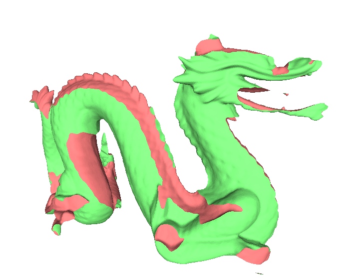
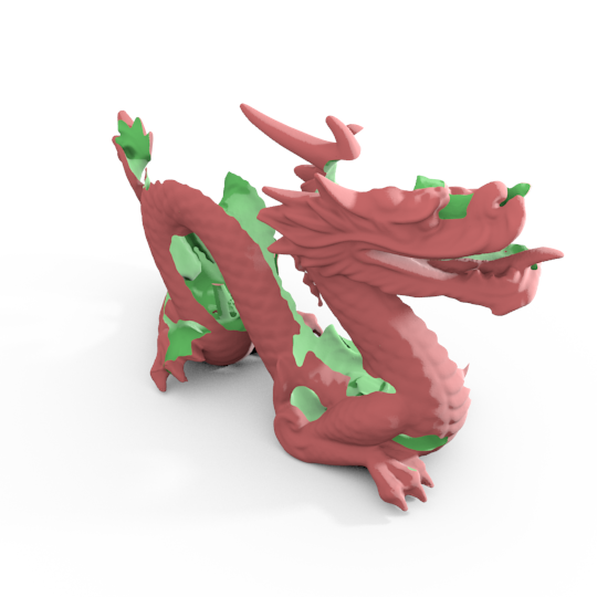
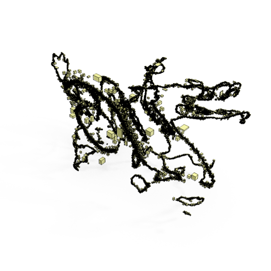
Results for the dragon example
The original model contains many small
holes, that are cause errors in the reconstruction. However, the reconstruction result still looks ok.
Result for intersection:
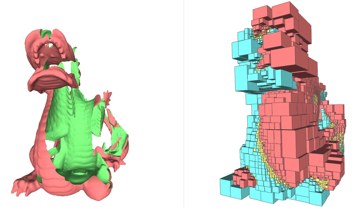
Result for difference, and leaves of the KD-tree (reddish = suppressed nodes, cyan = copied without processing, yellow = where QuickCSG searched for double and triple vertices)
Other viewpoint (result, kdtree, only yellow nodes of kdtree):
./mesh_csg data/feito2013/{dragon_vrip,dragon_transformed}.off -union -o /tmp/dragon_union.off -tess -v 1111111111
Loading data/feito2013/dragon_vrip.off (off)
Loading data/feito2013/dragon_transformed.off (off)
  Load input 2248.035 ms
  2 meshes, 875290 vertices, 1742828 facets
Register edge-facet links
  topology time 402.507 ms
KDTree to vertices
  exploration in 648.680 ms
Building output facets
  facet time 220.860 ms
Encountered errors during CSG computation:
  318 times makeFacet: could not find closed loop
  7 times addHEPairsPrimary: primary vertex from < 3 facets on output mesh
  177 times makeFacetOnlyPrimaries: not same nb of primary vertices as in input
Storing output /tmp/dragon_union.off
  output time 2021.448 ms


./mesh_csg data/feito2013/{dragon_vrip,dragon_transformed}.off -inter -o /tmp/dragon_inter.off -tess -v 1111111111
Loading data/feito2013/dragon_vrip.off (off)
Loading data/feito2013/dragon_transformed.off (off)
  Load input 2236.206 ms
  2 meshes, 875290 vertices, 1742828 facets
Register edge-facet links
  topology time 401.791 ms
KDTree to vertices
  exploration in 629.162 ms
Building output facets
  facet time 173.812 ms
Encountered errors during CSG computation:
  305 times makeFacet: could not find closed loop
  23 times addHEPairsPrimary: primary vertex from < 3 facets on output mesh
  169 times makeFacetOnlyPrimaries: not same nb of primary vertices as in input
Storing output /tmp/dragon_inter.off
  output time 1198.152 ms


./mesh_csg data/feito2013/{dragon_vrip,dragon_transformed}.off -diff 1 -o /tmp/dragon_diff.off -tess -v 1111111111
Loading data/feito2013/dragon_vrip.off (off)
Loading data/feito2013/dragon_transformed.off (off)
  Load input 2222.924 ms
  2 meshes, 875290 vertices, 1742828 facets
Register edge-facet links
  topology time 401.967 ms
KDTree to vertices
  exploration in 642.111 ms
Building output facets
  facet time 196.047 ms
Encountered errors during CSG computation:
  321 times makeFacet: could not find closed loop
  176 times makeFacetOnlyPrimaries: not same nb of primary vertices as in input
  5 times addHEPairsPrimary: primary vertex from < 3 facets on output mesh
Storing output /tmp/dragon_diff.off
  output time 1590.660 ms

./mesh_csg data/feito2013/{dragon_transformed,dragon_vrip}.off -diff 1 -o /tmp/dragon_rdiff.off -tess -v 1111111111
Loading data/feito2013/dragon_transformed.off (off)
Loading data/feito2013/dragon_vrip.off (off)
  Load input 2250.046 ms
  2 meshes, 875290 vertices, 1742828 facets
Register edge-facet links
  topology time 426.600 ms
KDTree to vertices
  exploration in 644.541 ms
Building output facets
  facet time 198.684 ms
Encountered errors during CSG computation:
  25 times addHEPairsPrimary: primary vertex from < 3 facets on output mesh
  318 times makeFacet: could not find closed loop
  170 times makeFacetOnlyPrimaries: not same nb of primary vertices as in input
Storing output /tmp/dragon_rdiff.off
  output time 1623.585 ms
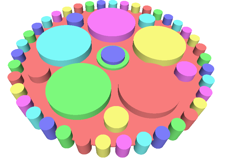
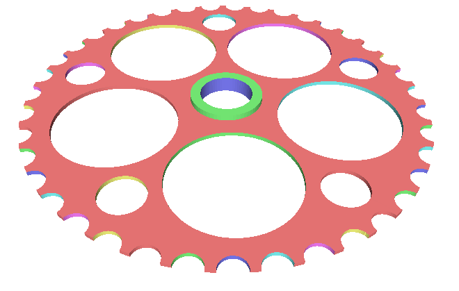
Use option -kdtree.save_off xx.off to output the kdtree.
Note that in this case we need -random.translation
and -random.rotation because the input configuration is
prone to degeneracies.
./mesh_csg -v 111111 -diff 2 data/hybrid_booleans/Sprocket/{0..51}.off -o /tmp/out.off -random.rotation -random.translation 1e-5 -tess

....
Loading data/hybrid_booleans/Sprocket/50.off (off)
Loading data/hybrid_booleans/Sprocket/51.off (off)
  Load input 18.017 ms
  52 meshes, 6008 vertices, 11808 facets
Applying random perturbation
  Preprocessing time: 0.066 ms
Register edge-facet links
  topology time 2.165 ms
KDTree to vertices
  exploration in 18.621 ms
Building output facets
  facet time 9.758 ms
Storing output /tmp/out.off
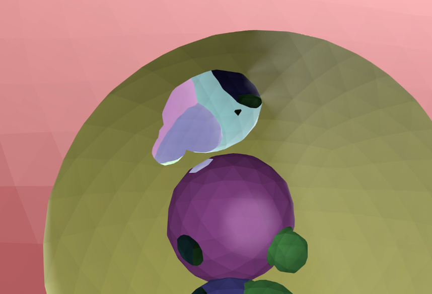
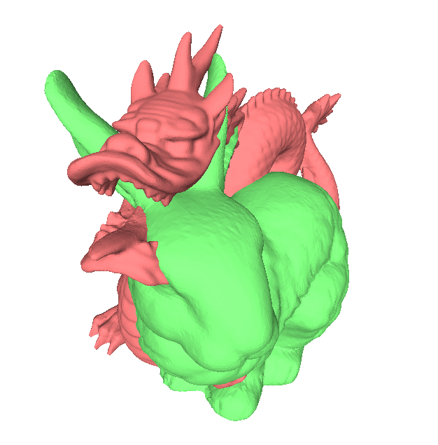
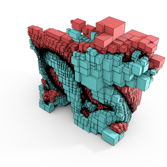
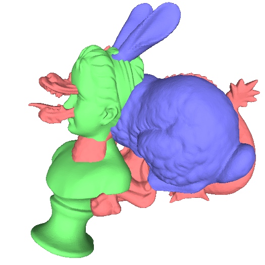
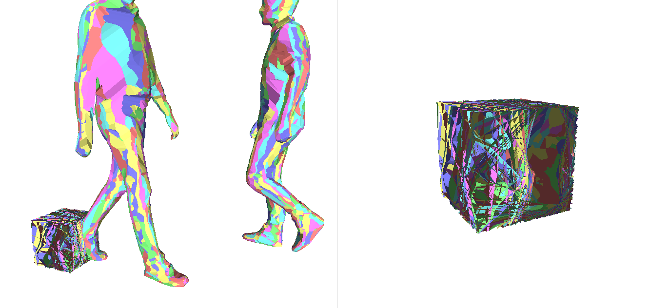
Organic
This is a 6-mesh dataset where 3 boxes are subtracted from 3 meshes (a
dragon, a bunny and a head), and the cropped meshes are merged into one result.
The meshes are available here: organic.tgz.
The input data was put together with the help of Marcel Campen. Thanks Marcel!
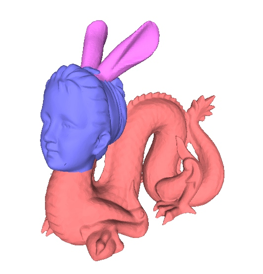
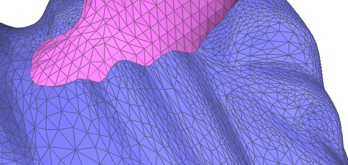
Inputs (without the cropping boxes, that would clutter the image):
Output + close-up that shows the intersecting area between the ears and the head. There is no additional geometry due to tesselization (QuickCSG only tesselizes non-convex output polygons):
./mesh_csg -csgprog '01-23-45-||' data/hybrid_booleans/Organic/{orig/0.off,dragon_box.off,orig/1.off,head_box.off,bunny_remap.off,ears_box.off} -combined /tmp/combined.off -o /tmp/out.off -v 11111111 -tess -parallel.nt 1
Loading data/hybrid_booleans/Organic/orig/0.off (off)
Loading data/hybrid_booleans/Organic/dragon_box.off (off)
Loading data/hybrid_booleans/Organic/orig/1.off (off)
Loading data/hybrid_booleans/Organic/head_box.off (off)
Loading data/hybrid_booleans/Organic/bunny_remap.off (off)
Loading data/hybrid_booleans/Organic/ears_box.off (off)
  Load input 284.876 ms
  6 meshes, 112043 vertices, 219244 facets
Register edge-facet links
  topology time 98.946 ms
storing combined meshes to /tmp/combined.off
KDTree to vertices
  exploration in 323.594 ms
Building output facets
  facet time 63.789 ms
Storing output /tmp/out.off
  output time 235.503 ms
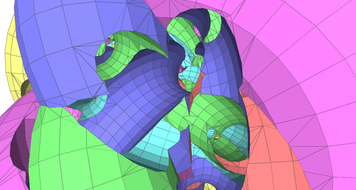
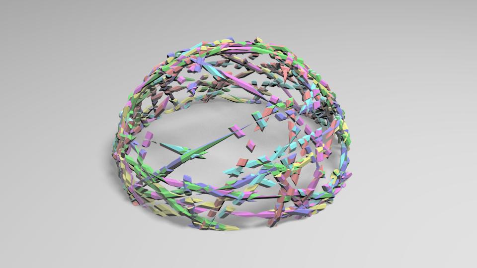
EPVH
Like the example H, kino68 is a visual hull-based reconstruction. However, in this case, it is possible to reconstuct the result more efficiently by not creating and processing the basis of the cones, so we start at a root node that contains cropped polygons. Note that the examples below are computed on 60 out of the 68 available silhouettes because the executable supports a limited nb of inputs.
kdtree node somewhere in the middle of the reconstruction:
mkCSG $ ./mesh_csg -contours data/capture_kinovis/CONTOURS/contour-00426.oc data/capture_kinovis/68cam.calib -o /tmp/out.off -v 1111111 -cropbbox -10,-10,-10,10,10,10  -contourdepth 40 -random.jitter 0.0001 -contourrange 0,60
  Load contours 36.127 ms
  60 meshes, 40223 vertices, 39470 facets
Cropping root node to provided bbox
  time 3.551 ms
KDTree to vertices
  exploration in 542.814 ms
Building output facets
  facet time 9.113 ms
Storing output /tmp/out.off

# select a node in the hierachy

./mesh_csg -contours data/capture_kinovis/CONTOURS/contour-00426.oc data/capture_kinovis/68cam.calib -o /tmp/out.off -v 11111111 -cropbbox -10,-10,-10,10,10,10  -contourdepth 40 -random.jitter 0.0001 -contourrange 0,60 -savenode '<211212212221221211>' /tmp/node.off
  Load contours 45.491 ms
  60 meshes, 40223 vertices, 39470 facets
Cropping root node to provided bbox
  time 6.441 ms
KDTree to vertices
storing node <211212212221221211> to /tmp/node.off
  exploration in 885.052 ms
Building output facets
  facet time 15.153 ms
Storing output /tmp/out.off
  output time 48.512 ms
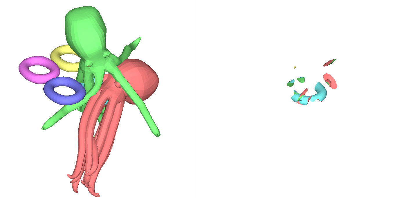
./mesh_csg -min2 data/poulpe/{4..9}_*.off -combined data/poulpe/combined.off -o data/poulpe/min2.off -v 11111111
Loading data/poulpe/4_Visual.off
Loading data/poulpe/5_Visual.off
Loading data/poulpe/6_model.off
Loading data/poulpe/7_model.off
Loading data/poulpe/8_model.off
Loading data/poulpe/9_model.off
  Load input 42.463 ms
  6 meshes, 16524 vertices, 33040 facets
Register edge-facet links
  time 5.654 ms
storing combined meshes to data/poulpe/combined.off
KDTree to vertices
  exploration in 13.749 ms
Building output facets
  facet time 1.813 ms
Storing output data/poulpe/min2.off
  output time 4.753 ms
Extreme CSG
Here we are pushing the limits of what can be done with CSG operations.
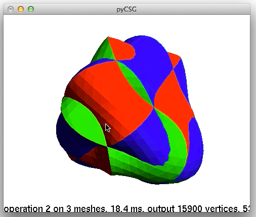
Real-time CSG
Video capture of a real-time CSG application, where a 3 series of boxes are
used as input for several CSG operations:
.
Same idea: 3 bumpy spheres rotate indpendently:
.
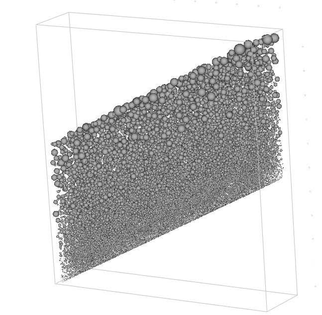
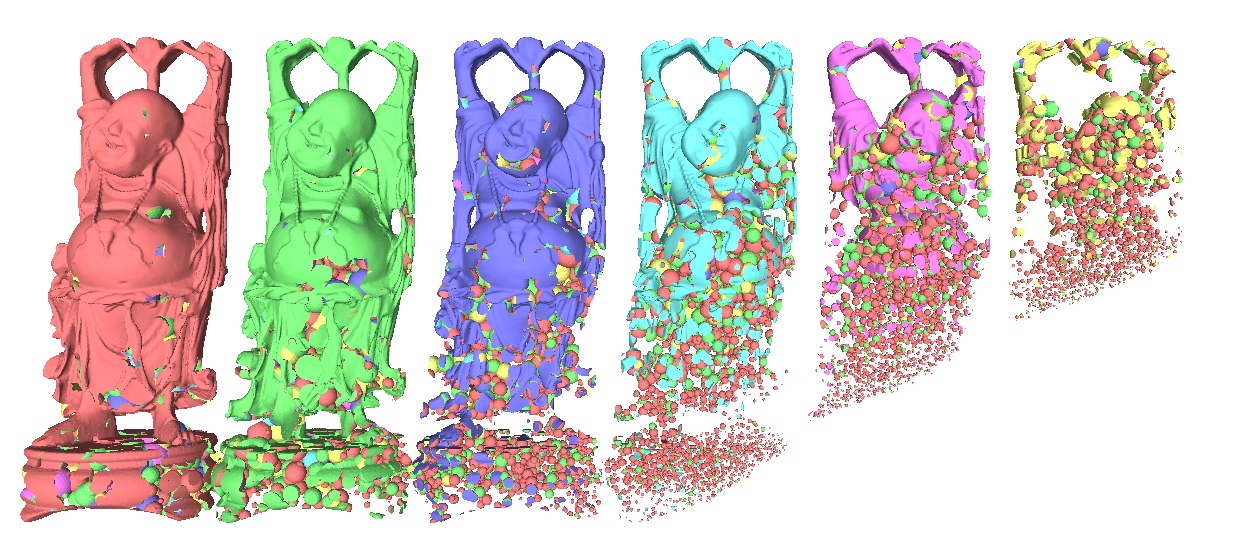
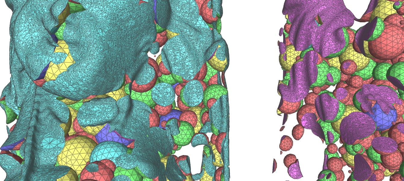
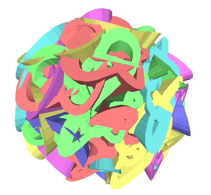
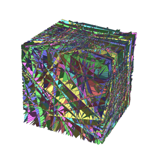
The 6 Buddhas
It combines six instances of the "Happy Buddha"
the largest mesh from the Stanford
repository. We intersect these with the union of 100,000 random spheres.
The spheres were labeled with
a greedy graph coloring algorithm to group them into 37 disjoint
subsets, so there are a total of 43 input meshes.
experiments $ ../mesh_csg -dither data/dither/{dragt,dragt2,box,yy_0,yy_1,yy_2}.off -random.translation 1e-4 -random.rotation -v 11111111 -tess -o /tmp/out.off
Loading data/dither/dragt.off (off)
Loading data/dither/dragt2.off (off)
Loading data/dither/box.off (off)
Loading data/dither/yy_0.off (off)
Loading data/dither/yy_1.off (off)
Loading data/dither/yy_2.off (off)
  Load input 2076.741 ms
  6 meshes, 876298 vertices, 1743634 facets
Applying random perturbation
  Preprocessing time: 11.198 ms
Register edge-facet links
  topology time 368.532 ms
KDTree to vertices
  exploration in 1206.615 ms
Building output facets
  facet time 858.469 ms
Reverting random perturbation
  revert: 174.120 ms
Encountered errors during CSG computation:
  111 times addHEPairsPrimary: primary vertex from < 3 facets on output mesh
  1318 times makeFacet: could not find closed loop
  118 times makeFacetOnlyPrimaries: not same nb of primary vertices as in input
Storing output /tmp/out.off
  output time 3203.084 ms
Dark star
This example is built by subtracting random spheres from a large one until there is a
hollow path between the two sides of the large sphere. We generate an animation by
following the path with a camera and a light source.
Generated videos (seems to be readable only in Google Chrome):
Additional material
Here we reproduce a few images and some details that did not fit in the paper.
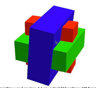
Viewing the KD-tree
On a simple example, it is possible to visualize the kdtree.
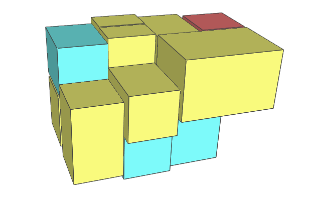
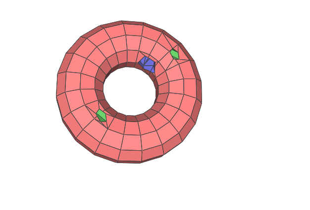
We compute operation Pf = P1 \ (P2 U P3) applied to three simple meshes (f.l.t.r: input, kdtree, output):
On the graph below, each box represents a node, whose width is proportional to its number of polygons. When space allows, text in the box indicates node's indicator vector and the number of polygons. Color code: ■ = node that was split, ■ = leaf where vertices were found with CSGVertices, ■ = facets were just copied to the output, ■ = nodewas found completely inside or outside the mesh. Each dashed box represents a parallel task.
Finding the orientation of a kdtree node
This document complements Section 6.3 of the paper, by giving some details of how the polyhedron's orientation w.r.t one direction can be computed in a single pass over its faces:
 (b)
(b)
 (c)
(c)
 .
.
 .
.